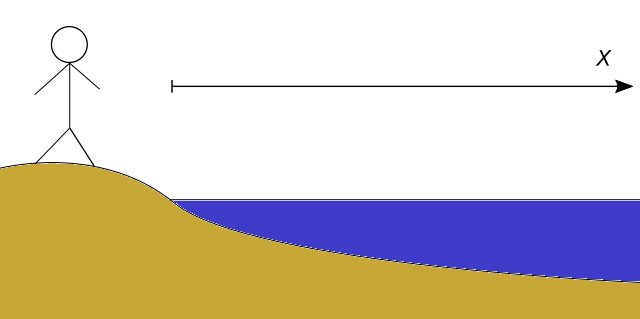
In the past summer, I spent several days at the beach with my daughter. There I had time to sit on the sand, watch the sea, watch her play in the shallow water, and occasionally rush to the sea to save some plastic toy from drifting.

But why do the toys drift? Floating objects drifting away from the shore is something everyone knows about, but I’ve never heard a satisfactory explanation why. On average, a body of water isn’t moving, so locally a floating object should move in either direction with equal probability. On a large scale, currents break this symmetry. But what about bodies in shallow water close to the shore? Surely such effects don’t play any role here.

I used to study physics at the university, so finding an explanation seemed like a fun exercise. I’ve never shined in fluid mechanics, so I wondered if I could find a simple model explaining this behavior.

Enter random walks

The movement of a toy on the water is essentially random. If you want to simulate stochastic movement without simulating the dynamics behind that movement, the most obvious place to look for is random walks. A random walk is an abstract mathematical object that takes successive steps in some mathematical space.

The simplest example of a random walk is one that happens in the one-dimensional number line. The walk starts at 0. Each iteration moves it by -1 or +1 with equal probability. The result is a zigzaggy movement that initially stays around 0 but starts to spread further and further away as time goes.

This model is simple enough to be exactly solvable. In particular, if \( X_n \) denotes the coordinate of the walk after \( n \) steps, we have \( \langle X_n \rangle = 0 \) and \( \langle X_n^2 \rangle = n \). The expectation value \( \langle X_n \rangle \) staying tells us that there isn't a preferred direction (what would it be?). The variance \( \langle X_n^2 \rangle \) being proportional to the time passed means that the standard deviation of the coordinate is proportional to the square root of the time. Moreover, thanks to the central limit theorem, we know that for large \( n \), the distribution of \( X_n \) starts to approach a normal distribution.

It means that a random walk tends to drift away from its initial position but slower and slower as time goes. The fact that a simple random walk on average drifts away from its initial position, while being completely symmetric locally, already hints that it's a useful model when explaining floating objects drifting toward the sea.

Random walks at the shoreline

Let’s model the plastic toy at the beach as a random walk. Le’s set the one-dimensional coordinates so that the beach extends to the negative X-axis, the sea to the positive X-axis, and the toy is initially at 0 right where the water meets the shore.

At each iteration, the toy moves toward or away from the sea with equal probability. The only difference to the simple random walk is that a toy cannot move to the sand. So if the coordinate is already 0, it will not decrease.

Since my pen-and-paper routine is rusty, I decided to write a program to simulate lots and lots of walks. The source code is available on GitHub. Running lots of random walks of varying timespans gives a relation between the expected distance to the beach as a function of time:

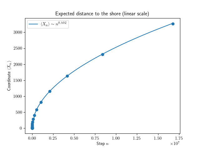
We see that, unsurprisingly, as more time passes, the expectation value increases. Something even more interesting is visible when plotting the above data on a logarithmic scale:

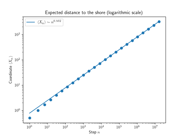
We see that (in this particular simulation run) \( \log \langle X_n \rangle \sim 0.502 \log n \), which gives a functional relation \( \langle X_n \rangle \sim n^{0.502} \approx \sqrt n \). A relation that has form \( y \sim x^\alpha \) for some \( \alpha \) is called a power law, and finding one tends to make a phycisit happy.

Why does a toy drift?

We can interpret the above result as follows: Although the toy is as likely to move toward the shore as away from it, the distance you expect to find it increases as time passes. Thus it becomes increasingly rare that the object drifts back to the shore.

The fact that the drift is related to the time by a power law also hints that the drifting is scale-invariant. If we measure the distance of the toy with a yardstick twice the length, and a clock ticking at a quarter of the rate, we measure the same behavior.

The scale invariance gives the motion a fractal-like behavior, where the path on a small scale is self-similar to itself on a large scale. These ideas provide mathematical tools to reason about many phenomena in statistical mechanics and quantum field theory. Pretty deep, considering we were studying a plastic toy at a beach!

Hindsight

I said earlier that I decided to simulate since my pen-and-paper routine is admittedly rusty. But the functional form made me wonder if the problem was so challenging after all. When looking at the distribution of the coordinate after \( 2^{24} \) steps, this is what happens:

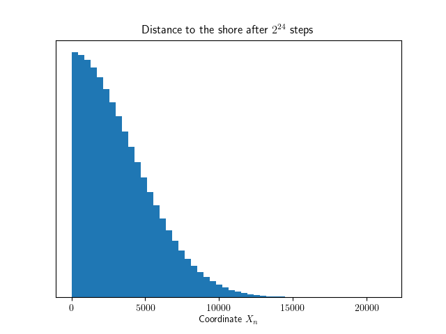
Yup, it's the right half of a normal distribution. And that makes sense: The only difference between the simple random walk and our random walk is the fact that our random walk is “reflected” when trying to enter the negative x-axis. But since the normal distribution is symmetric, this merely restricts the original normal distribution to the positive axis.

The nice thing about the one-sided normal distribution is that we can calculate the expectation value using integration by substitution. Recall the probability density of the normal distribution, and that \( \sigma^2 = n \). Then by substitution \( u = x^2/n \) we have:

\[ \langle X_n \rangle = \int_0^\infty \frac{2}{\sqrt{2\pi n}}e^{-\frac{x^2}{n}} x \mathrm d x = \sqrt \frac{n}{2\pi} \int_0^\infty e^{-u} \mathrm d u = \sqrt \frac{n}{2\pi} \]

Boom! Varying an old programming joke about debugging and reading the documentation: Six hours of writing a simulation program can save you five minutes of pen-and-paper calculation.